
Some background
Formal literature on property, or real estate, cycles have only been published over the past 30-odd years and most of it relating to the US and UK real estate markets. The theme of real estate cycles is part of the broader ‘economics of the real estate market’. The latter encompasses a number of activities, ranging from institutional aspects (e.g. real estate developers, investors, construction companies, financial institutions, service providers, users, etc.) to management aspects (e.g. portfolio management, real estate analysis, appraisal, finance, marketing, project development, construction project management and facilities management) and topological aspects (e.g. commercial real estate, residential real estate, industrial real estate and special real estate). It follows that real estate economics have interdisciplinary interfaces, e.g. economics, architecture, engineering, law and spatial planning (see Rotke et al, 2003: 328)
The objective of the current note is to outline the basic features of the property cycle. To that effect, we differentiate between real estate, e.g. residential housing, commercial property (including shopping, banking and office space), industrial space (manufacturing and whare-housing) and the building & construction market. While these market segments fall under the ‘economics of the real estate market’, their cyclical dynamics differ. The construction cycle is discussed elsewhere. The focus in the current note is on the property cycle, i.e. the housing and the commercial and industrial rental markets.
The general business cycle is invisible but real. In essence, the business cycle involves successive periods of economic acceleration/ expansion followed by slowdown or contraction in unceasing rounds. The interaction of macro-economic magnitudes at the turning points teaches us much about the nature and characteristics of business cycles. The real estate cycle forms part of the general business cycle, with a prominent lag relationship. In the general economy, business cycles typically have two sources, either endogenously due to macroeconomic imbalances, or exogenously, due to external and discrete shocks (see Ewing & Hawkins, 2007: 32). In the property sector, endogenous cycles typically occur due to frictions arising from various lags, apart from the exogenous influences at the macroeconomic level.
Sources of the property cycle
Regarding endogenous sources of the property cycle, Rode & Associates point out that a general lag exists of between 1 and 2 years with the general business cycle. At the bottom of the cycle, it is typically a situation over over-supply that needs to be cleared, causing the property cycle to lag the general business cycle; conversely, at the peak of the cycle, shortages exist, which need to be supplied. Rotke et al (2003) dissects this long delay in property cyclical turning points further, referring to three important lags. Firstly, the lag tied to the price-mechanism; secondly, the decision lag; and finally, the construction lag.
Regarding the price-mechanism lag, the issue is that when demand increases (unexpectedly), vacancies first need to decline, whilst the space availability is fixed (in the short term). The consequence is that prices increase (e.g. rentals). Rentals would be the signal for property developers and construction companies to increase the supply. However, vacancy rates first have to reach the so-called ‘natural level’ and rentals to increase sufficiently to signal the need for additional space. The second phase of the lag relates to decision time involved in identifying and planning a property development (i.e. the investment decision). These could be large projects requiring finance and big construction companies having to design and deliver the additional space. The third and final phase of the lag relates to the actual construction of the property development – in residential housing, this could be anything from 6-12 months and longer; in the non-residential sector, a similar lag or longer is very likely.
Apart from the endogenous sources of the property cycle, exogenous influences may also be at play. In fact, being a sector, the initial trigger for the (endogenous) property cycle described above typically tends to be outside of the property sector itself, i.e. in the macro domain. Triggers such as demand changes/shocks driven by macroeconomic imbalances correcting (characterised by movements in interest and exchange rates, inflation and economic growth); the impact of droughts in agriculture; political instability and wars, etc. will all impact the property sector exogenously. Some external influences can evolve over time, rendering medium- to longer term impacts, e.g. structural changes (environmental change; political change and upheaval; technological change, leading to space-time changes, etc.). Beyond these exogenous factors, the property sector is faced with the reality of behavioural characteristics of the key role players in the sector (see Rotke et al, 2003: 331).
Methodological notes
As noted, the property cycle – as the general business cycle – is invisible. The question is how one can obtain a handle on it? In the choice between one property sector variable as a reference indicator of the property cycle, such as ‘all-property returns’, or the consideration of a number of time series’ stylized facts (e.g. first and higher order moments, lead & lags, etc.), BCA opted for the latter. This approach boils down to the description of several property variables and their coincident movements rather than only the consideration of a single ‘reference variable’. As such it is hoped to learn more of the multi-faceted property cycle.
An analysis of the property cycle commences with a methodology to date (determine, assess) the general business cycle. In this regard, both GDP and the SARB’s coincident economic indicator were used in determining general business cycle turning points by, first, applying a Christiano-Fitzgerald (CF) band pass filter (to remove the trend and establish a reference business cycle time series) and, second, a Bry-Boschan quarterly algorithm (BBQ) to date the turning points in this reference series[1].
The same methodology was applied to the property sector variables, i.e. real house prices (a reference series for the residential market), real office rentals (a reference series for the commercial market) and real industrial rentals (a reference series for the industrial market). Finally, an assessment of building contractor margins was also included in the analysis, interrogating the link with the construction market.
An analysis of these property variables provides a relatively comprehensive representation of the property cycle in SA, including a consideration of the trajectory of building profit margins. A distinction was also drawn between the shorter-term and medium-to longer term trajectories of the property cycle. A rich body of literature points to the medium-to longer term nature of the real estate cycle, lasting between 18-20 years. Rode & Associates reports a typical trough-to-trough real estate cycle in the SA economy lasting around 17 years (Rode’s SA Property Trends, December 2020: 12). This research institute also identifies on average two general business cycles in one property cycle. BCA’s analysis of the property cycle concurs with this knowledge developed in practice.
It is important to be aware of the property cycle in order to conduct efficient business planning and financial management. The reality is that even with detailed information and analysis of past cycles, it remains a challenge to accurately anticipate and plan for future cycles. Nonetheless, proper analysis of real estate cycles improves market transparency, underpins rational decision-making, which, in all, improve a property firm’s ability to navigate the cycle.
Considering the short- and medium-term SA property cycle
As noted, a main feature of the property cycle is its medium-term nature. A shorter cycle is identifiable, which also corresponds with the general high-frequency business cycle; however, the medium-term property cycle is of particular interest. A property sector business cycle (typically 15-20 years) can span two general business cycles (typically 8-10 years) in SA[2]. This is a stylized fact regarding the SA property cycle (see Rode’s Property Trends, December 2020: 12) and will be investigated in the current exercise.
In order to identify the property cycle, four property variables: (1) house prices (2) office rentals (3) industrial rentals; and (4) contractor margins will be analysed. These four property time series will be deflated by applying two price indices, i.e. (1) the BER building cost index (BERBCI); and (2) Statistics SA’s Haylett180 index, tracking building material costs. The nominal property sector variables will also be considered.
Regarding, the methodology applied to identify the property cycle, it is necessary to highlight the fact that changes in the trend and cycle of an economic time series are interactive and interdependent. By ‘removing’ the trend from a time series (e.g. applying a filter), this could lead to a loss of information on the true business cycle. This has led to fierce criticism of the use of deviation business cycle analysis (Harding & Pagan, 2005).
However, leading business cycle researchers acknowledge this, but do point out that frequency filtering may be considered for historical business cycle analysis (See Boshoff & McLean, 2018; Zarnowitz & Ozylidirim, 2001). This will be the focus in the current exercise. Furthermore, extracting the medium-term cycle – as opposed to the high-frequency cycle – with frequency filtering appears to be closer to the truth (Boshoff & McLean, 2018). This is a particular interesting prospect in terms of the generally accepted longer property cycle.
The methodology applied here, therefore boils down to calculating the (normalized) deviation cycles using a Christiano-Fitzgerald (CF) band pass filter. Both high-frequency (1.5 to 8 years) and low-frequency (1.5 to 50 years) deviation cycles are considered. Once the deviation cycle has been separated from the trend, business cycle turning points are determined using the BBQ algorithm.
Finally, the business cycle phases are mapped and the lead & lag patterns are considered (using cross correlograms) versus the GDP deviation cycle (as well as the CEI deviation cycle in order to test the robustness of the results). The highest correlations in respect of each property variable and the optimum lead/lagged GDP deviation cycle are established. The analysis excludes the COVID-19 impact, with the sample period being 1975Q1 to 2019Q4.
The business cycle can be expressed as follows:
Δyt = Δτt + Δct + εt
Where: Δyt = change in GDP, period t-1 to period t
Δτt = change in the trend component
Δct = change in the cyclical component
εt = random disturbance
Applying the CF band pass filter, economic fluctuations with frequency less than 1.5 years (6 quarters) are excluded from the cyclical component, Δct (considered part of the random disturbance, εt); as well as excluding those with frequency more than 8 years (32 quarters). This leaves us with the high-frequency business cycle.
Fluctuations with frequency between 32 (8 years) and 200 quarters (50 years) are considered as part of the medium-term component, say Δm’ct therefore:
Δyt = Δτ’t + (Δm’ct + Δc’t) + ε’t
Where: (Δm’ct + Δc’t) = medium-term cycle (or the low-frequency cycle)
When the change in an economic time series, e.g. GDP, is therefore decomposed into its trend and cycle components and we consider the business cycle as the ‘deviation from trend’, then:
- An economic downturn should be seen as a period where the growth rate is ‘below-trend’ (negative output gap) à either moving away from trend (accelerating downturn) or moving towards trend (decelerating downturn).
- An economic upturn, where growth is ‘above-trend’ (positive output gap) à either moving away from trend (accelerating upturn), or moving towards trend (decelerating upturn).
The medium-term cycle includes the economic fluctuations with frequencies between 1.5 and 50 years. Frequencies < 1.5 years are considered as part of the random disturbance and frequencies > 50 years as part of the trend. Given the unique length of property cycles, it makes sense to extract the medium-term cycle from property data. In all, in order to determine the high-frequency (or short-term) cycle, the CF filter parameters are set such that only fluctuations with a frequency between 1.5 and 8 years (or 6 and 32 quarters) are measured. For identifying the medium-term cycle the corresponding parameters will measure fluctuations of between 8 and 50 years (or 32 and 200 quarters). In the first part below, the high-frequency property cycle is considered.
The housing market
The SA housing market witnessed a peak during the early 1980s and a drawn-out downturn subsequently, which only bottomed at the time of the political transition to a full democracy (1994). In fact, the trough was registered in 1996/97, making it a long trough – see charts left. Thereafter, the sector witnessed a powerful upturn as the first post-apartheid economic recovery gathered momentum. The official general economic upturn between 1999 and 2007 became the longest in recorded SA economic history and nominal house prices increased six-fold over this period. The general property cycle peaked towards the end of 2008 (house prices in 2007). The housing market has since been in a downturn phase, with real house prices tapering lower (chart bottom, left).


Source: Rode & Associates / BCA
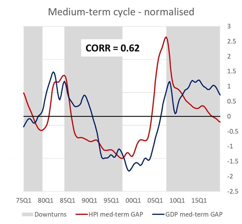
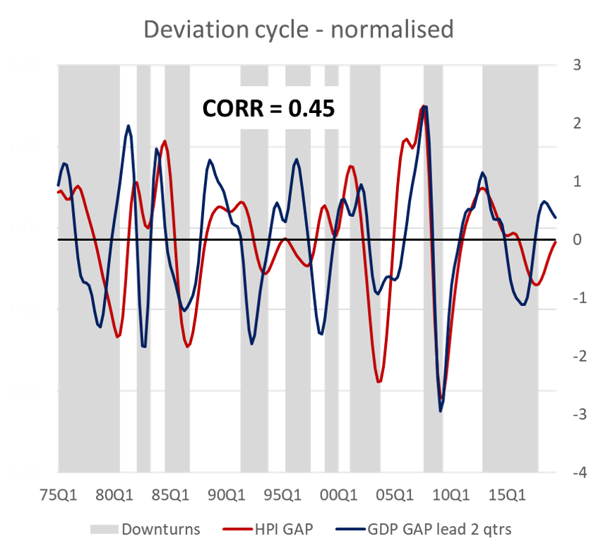
In Figure 1, both the high and low frequency housing price deviation cycles (HPI GAP) are depicted and correlated with the corresponding GDP deviation cycles (see charts right) . Cross correlation indicates that, over the short-term, the house price index (HPI) leads the GDP cycle by 2 quarters (6 months), including a reasonable positive correlation of 0.45 . House prices therefore tend to react early in the general economic cycle and generally moves with the business cycle. During the 1990s the correlation broke down somewhat (see chart top, right) due to structural change in the SA economy. From 1989 real interest rates were kept at high levels with the onset of a drive by the SARB to get inflation down. This temporarily distorted the relationship between real estate cycle and the economy-wide business cycle (see Rode’s Property Trends, December 2020: 15).
The medium-term house price cycle is substantially longer, with the duration of contraction phases averaging 39 quarters (i.e. close to 10 years) and expansion phases 31 quarters (i.e. close to 8 years). In line with the stylized facts regarding the SA housing price cycle, the full length of the medium-term cycle is close to 18 years. Cross correlation indicates the medium-term HPI coincides with the GDP med-term cycle and the correlation (1975-2019) is estimated at fairly strong 0.62.
The office market
SA’s office market (represented here by real office rentals in the Johannesburg node, ORJHB)) also witnessed a sharp peak during the early 1980s. Subsequently, real office rentals dropped sharply, establishing a long trough (1989-96). This market segment did recover subsequently, peaking in 2001. This was a short and mild upturn and somewhat counter-cyclical. The national economy witnessed a sustained upturn over the period 1999 to 2007; however, during the initial phase of this upturn, spending levels remained weak until 2002-03. Excluding the mild upturn in the office market (1997-2001), real JHB office rentals remained relatively flat over three decades (i.e. the 1990s, 2000s and 2010s) – see Figure 2 (charts, bottom).
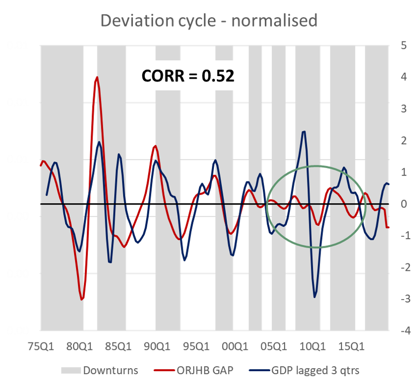
Figure 2 depicts both the high and low frequency real office rental deviation cycles (ORJHB GAP) and are correlated with the corresponding GDP deviation cycles (see charts right). Cross correlation indicates that real office rentals lag the GDP cycle by 3 quarters (9 months) over the short term. The reason for the lag was noted, namely that slack first needs to be taken up as the economy turns (meaning vacancy rates need to decline to its natural level) before rentals will start increasing (and vice versa during an economic downturn). Furthermore, correlation (1975-2019) improves from 0.37 to 0.52 when nominal office rentals are deflated by Haylett 180 (i.e. excluding contractor margins). This is a reasonable correlation, albeit evident that the office market was left relatively unscathed by the GFC (2008-09), presumably due to the fact that SA’s financial markets were not overly disrupted by the global instability at the time.
The longer-term analysis shows that the average downturn in real office rentals lasted 22 quarters (or 5½ years) and the average upturn, 31 quarters (or close to 8 years), suggesting a full-length medium-term office rental cycle of 13-14 years. Real office rentals are poorly correlated with the medium-term GDP cycle (lagged 4 quarters); correlation (1975-2019) is estimated at 0.23.



The industrial market
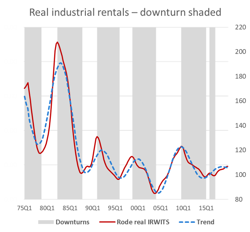
The industrial rental market (represented here by real industrial rentals in the Witwatersrand node, IRWITS) shows a similar cycle compared to the office market. It also witnessed a high peak during the early 1980s and while there have been shorter cycles subsequently, the trend in real industrial rentals have been downwards. A notable feature of the industrial market is the narrowing of the cycle amplitudes, particularly over the period from the 1990s. Furthermore, this property sector did benefit from the broader historically strong economic expansion between 1999 and 2007, albeit with a considerable lag. The industrial market witnessed a relative strong cyclical upswing from around 2003 to 2009. The general economic momentum also gathered pace from around 2002-03.
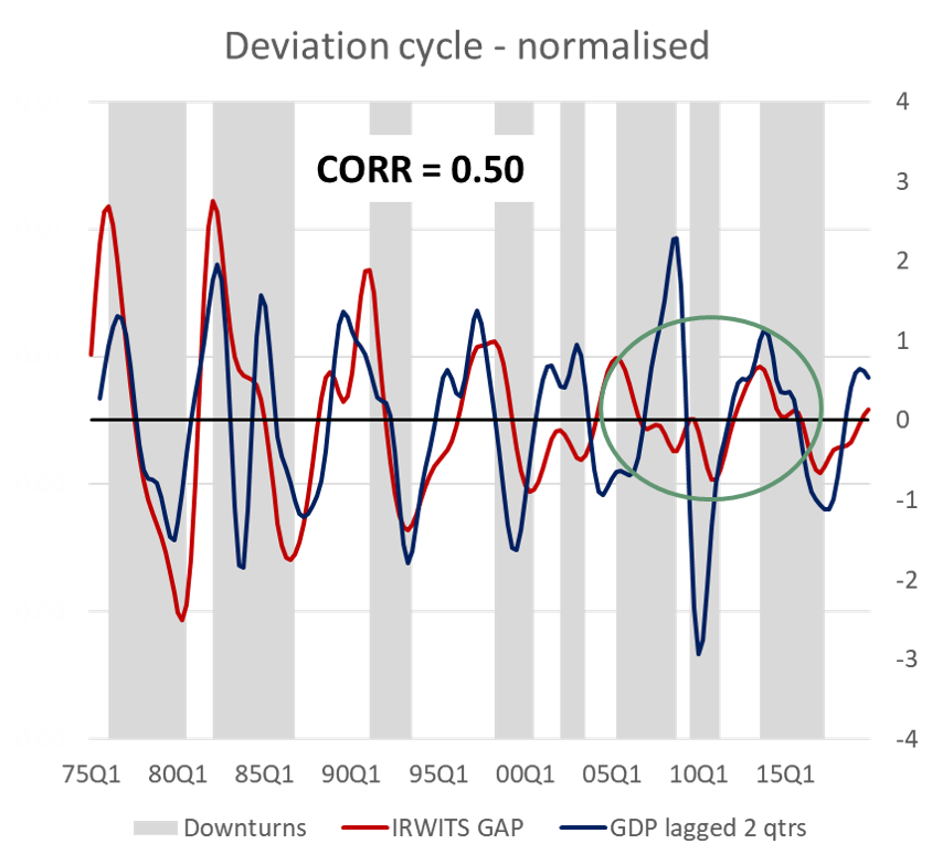
Figure 3 depicts both the short-term and the medium-term industrial rental deviation cycle compared to the GDP deviation cycle over the period 1975 to 2019 (charts, right). Over the short-term the correlation is reasonably strong and positive, i.e. 0.50. As was the case in the office market, the industrial market also does not share the volatility in overall real economic activity over the 2008-09 period at the time of the GFC impact. This is interesting as the local manufacturing sector did take a huge hit via its extensive trade channels.
The industrial market does reveal a slightly shorter lag with the general business cycle (represented here by the GDP deviation cycle), namely 2 quarters (or 6 months). The short lag would be consistent with the fact that manufacturing output tends to coincide with movements in GDP (or the general business cycle).
Source: Rode & Associates / BCA
Over the medium-term, the correlation coefficient (1975-2019) is 0.42, which is also reasonable, albeit that it is on the weak side. It also needs to be noted that the best-fitting lag is a full calendar year. In terms of duration, the average downturn phase is 27 quarters (or 7 years) and the average upturn phase, 18 quarters (or 4½ years. This translates to a full cycle of 11-12 years.
Linking with the construction sector – contractor margins
In the literature, property returns are often taken as the appropriate and comprehensive reference variable for the general property cycle. While property returns are a function of property development costs, rentals and selling prices, contractor margins in the building and construction sector may also be an interesting reference variable for the property cycle. When general economic conditions are tight, tendering competition will tend to intensify, putting downward pressure on contractor margins and conversely during lively economic conditions.

Source: Statistics SA / BER / BCA
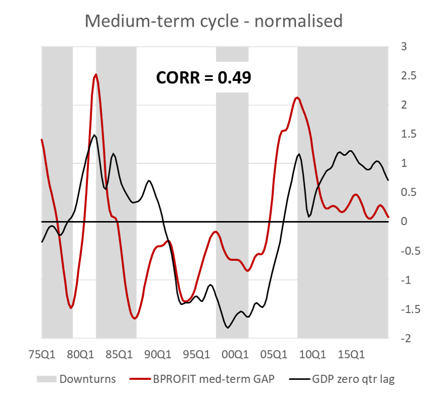
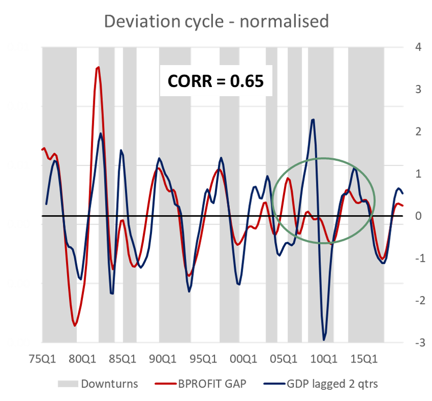
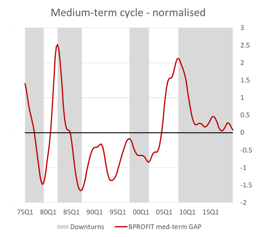
In Figure 4, the trajectory of building contractor margins is depicted by the ratio of the BER’s building cost index (including contractor margins) and Stats SA’s Haylett180 formula of building costs (excluding contractor margins). The cycle in contractor margins (or building profits, BPROFIT) is shown over both the short- and the longer-term. The building profit cycle broadly corresponds to that of the other property variables as one would expect. Margins are higher when house prices, or office and industrial rents, are high during an economic upturn; conversely, they come under pressure during an economic downturn.
Cross correlation indicates contractor margins lag the GDP deviation cycle by 2 quarters (6 months), with the correlation (1975-2019) with GDP is estimated at 0.65. This is a relatively strong positive correlation. The other interesting fact is that building profits are also well correlated with office and industrial rentals. This reflects the link between the property development side and actual selling or rental market.
The bottom charts in Figure 4 also show the medium-term cycle in contractor margins. The average duration of upswings in contractor margins is 27 quarters (or close to 7 years) and the downswing phases 25 quarters (or slightly more than 6 years). This suggests a full cycle duration of around 13 years. Contractor margins have a reasonable correlation with the medium-term GDP cycle (measured at 0.49), as well as with real house prices, real office and industrial rentals.
Considering the nominal property variables – the medium-term cycle
Real property variables are derived by deflating their nominal counterparts with the BER’s building cost index or Statistics SA’s Haylett180 formula. Deflating by the building cost index ‘removes’ an important cyclical magnitude, i.e., contractor margins. Furthermore, deflation by Haylett180 may not entirely be the appropriate index to deflate property rental and house price data. This justifies to at least consider property cycles in nominal terms.
The same methodology was used, only applied to the nominal time series, namely house prices, office rentals in Johannesburg and industrial rentals in Witwatersrand (HPI / ORJHB / IRWITS). Only the low frequency cycles were considered and correlated with the SA medium-term cycle (GDP med term GAP).
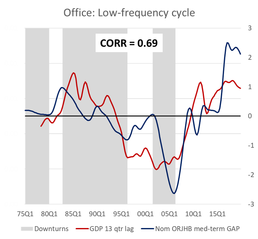
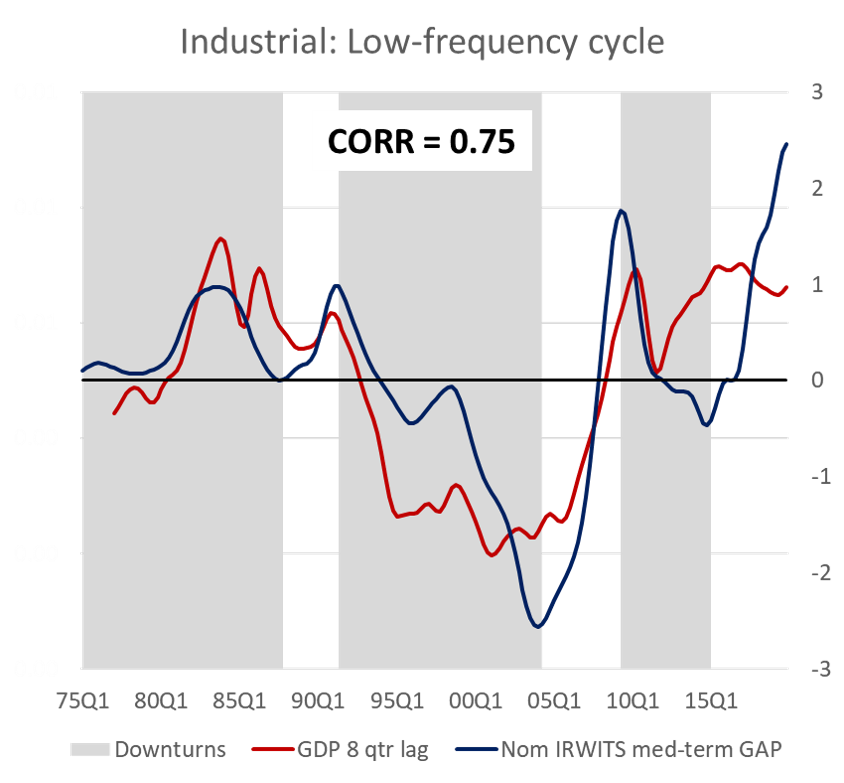
The overwhelming outcome was the improvement in the respective correlation coefficients. This suggest that there is some value in considering the nominal property variables. In the case of the housing market, the medium-term correlation improved from 0.62 to 0.65; in the case of office rentals, the correlation improved from 0.23 to 0.69 and regarding industrial rentals the corresponding number went from 0.42 to 0.75 – see Figure 5.
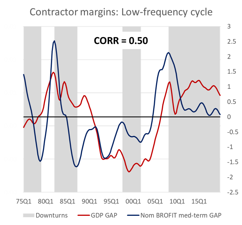
As contractor margins are by definition in nominal terms (i.e., the ratio between nominal building costs and the Haylett180 formula), its correlation with the medium-term GDP deviation cycle remains unchanged.
Finally, there are significant lags involved between turning points in the property variables and GDP. In the housing market, this lag was measured at 2 quarters (or six months), which is not long from a medium-term perspective. The lag is substantially longer in the case of the office market (13 quarters, or slightly more than 3 years) and the industrial market (8 quarters, or two years). Both the office and industrial market appears to be slow in adjusting to changing market conditions. This ties in with the nature of the real estate market.

Source: Rode & Associates / Statistics SA / BER / BCA
Turning point analysis
In the foregoing analysis, the lead/lag patterns were investigated for the individual property variables, including building contractor margins. One way to identify the turning points of the general property cycle, is to calculate the median of the tuning points of the individual property reference variables. As building contractor margins are more closely linked with building & construction as opposed to the property market conditions (housing, office and industrial space), it was decided to only include the three main property variables, i.e., real house prices, real office rentals (JHB) and real industrial rentals (WITS). By determining the median turning points, the turning points in the individual cyclical components of the three property variables are ‘integrated’. Interesting conclusions follow.
The method was applied, both in respect of the high- & low frequency cycles – see Table 1 and Table 2. Only the real values of the property variables were considered.

From Table 1, it is clear that the typical general (short-term) property cycle has a duration of 6.3 years (or 25 quarters), with downturns averaging 3 years (12 quarters) and upturns 3.3 years (15-16 quarters). Furthermore, the property cycle coincides with the GDP deviation cycle at peaks and lags it by 6 months (or 2 quarters) at troughs. This suggests that the general property cycle is broadly comparable to the national business cycle over the short term[4]. It should be noted that house prices tend to turn ahead of the general economy and may be the variable which counter the lags in office and industrial rentals, which results in a coincident median turning point in the general property cycle relative to the business cycle (GDP).
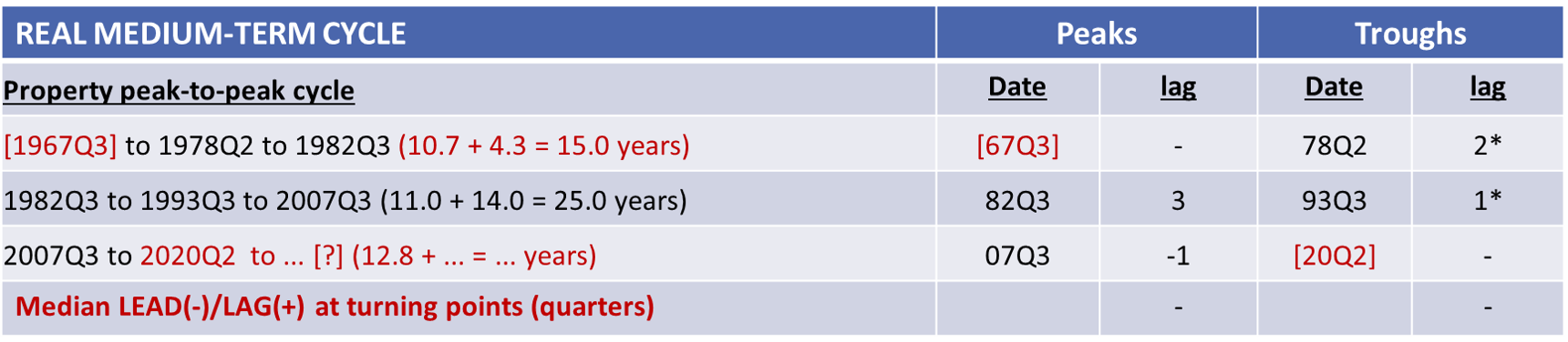
Considering the medium-term turning points in real house prices, office and industrial rentals, the following longer-term property cycle median turning points are identified:
- Peaks: cluster of upper turning points around 1982Q3 and 25 years later around 2007Q3; and
- Troughs: cluster of lower turning points around 1978Q2 and 15 years later around 1993Q3; the post-GFC lower turning point has not been identified (27 years later, 2020Q2?)
These medium-term turning points correspond to that of the national economy, albeit that the structural downturn in the broader economy has been dated earlier, i.e., the early- to mid-1970s. With the ascent of the gold price, peaking in 1980, and given the importance of gold export revenues in the economy at the time, this may have been an important driver of the housing and general property boom lasting up to the early-1980s. SA’s post-apartheid boom in the general property market delivered the next structural upper turning point in 2007. It should be noted that the spread of turning points is sometimes wide, particularly at the time of SA’s political transition – real industrial rentals troughed much earlier (1987) and real house prices much later (1997).
Concluding remarks
We have fairly consistent evidence that the property cycle in SA is closely linked with the national business cycle. This current analysis largely confirmed the stylized property cycle facts noted initially. In additional, some finer detail regarding the SA property cycle has been established. Broadly, the shorter-term property cycle lasts around 6½ years, comprising of a slightly shorter downturn phase on average compared to the upturn phase. The medium-term property cycle easily spans two full short cycles and is even longer in the case of the housing market. In all:
- The high-frequency property cycle is less consistent, with weaker co-movement with the general business cycle.
- The medium-term property cycle displays better co-movement with the national longer-term business cycle, with turning points coinciding for all practical purposes.
Regarding the individual property variables:
- Real house prices show average co-movement and tend to lead the business cycle (short-term); however, is well-correlated with the national medium-term cycle (coefficient of 0.62). The duration of the medium-term cycle is around 18 years, which agrees with Rode & Associates’ stylized fact of around 17 years. The analysis showed that downturns last slightly longer (10 years on average) and upturns, 8 years.
- Real office rentals also show average correlation (lagging 3-4 quarters) over the short-term and the medium-term cycle co-movement is worse (0.23), except when nominal rentals are considered. In terms of duration, the medium-term office rental cycle was measured between 13-14 years, with downturns averaging 5.5 years and upturns, close to 8 years.
- Real industrial rentals also show average correlation (0.42; lagging 2 quarters over the short-term and a full year over the medium-term). Nominal rentals show much better co-movement (0.70 correlation coefficient), also in the case of the medium-term cycle (0.75). The medium-term real industrial rental cycle lasts 11-12 years on average, with downturns averaging 7 years and upturns, a relatively short 4.5 years.
- Building contractor margins are well correlated with the general business cycle (short-term 0.65; lagging 2 quarters), with an average medium-term correlation of 0.49. The duration of the contractor margin cycle is similar to that of the office and industrial market, namely 13 years, with downturns averaging slightly more than 6 years and upturns, close to 7 years. The cycle in contractor margins also correlates reasonably well with that of real office or industrial rentals.
An interesting and useful result, is the fact that the nominal property variables show good co-movement, both short and longer term (except for margins that show average correlation longer term). The real property cycle is also closer to the truth when contractor margins are not included in the deflator, i.e., when Statistics SA’s Haylett180 formula of building cost is used to convert the nominal variables. This makes intuitive sense.
Finally, additional research is required, e.g., allowing for structural breaks; investigating different sample periods; and also considering alternative reference time series reflecting the property cycle, to name a few areas where the analysis can be refined.
References
- Boshoff, W.H. 2010: “Band-pass filters and business cycle analysis: High-frequency and medium-term deviation cycles in South Africa and what they measure”, Working Paper 200, Economic Research Southern Africa.
- Boshoff, WH & McLean, L. 2018: “What do deviation cycles measure? An analysis of the informational content of filter-based business cycles”, SA Journal of Economic & Management Sciences 21(1), a1689. https://doi.org/10.4102/sajems.v211.1689
- Burns, A.F. & Mitchell, W.C. 1946: Measuring Business Cycles, New York: National Bureau of Economic Research (NBER).
- Ewing, R. & Hawkins, J. 2007: “Business Cycles in Australia”, Paper presented to Australian Conference of Economists, Perth, September 2006 and, in revised form, to Australian Macroeconomics Workshop, April.
- Harding, D., & Pagan, A. 2005: “A Suggested Framework for Classifying the Modes of Cycle Research”, Journal of Applied Econometrics, 20(2), 151-159. Retrieved from http://www.jstor.org.ez.sun.ac.za/stable/25146349
- Rottke, N., Wernecke, M. & Schwartz, L. 2003. “Real Estate Cycles in Germany – Causes, Empirical Analysis and Recommendations for the Management of the Decision Process“, Journal of Real Estate Literature, Volume 11(3).
- Zarnowitz, V. & Ozyildirim, A. 2001: “Time series decomposition and measurement of business cycles, trends and growth cycles,” Economics Program Working Paper Series, EPWP #01-03. Conference Board, USA.
[5] Not shown here, are the results regarding the nominal property cycle. These results broadly agree with those reported here.
[3] It is important to note that whereas the GDP deviation cycle, calculated using the methodology described in the current exercise, generally agrees with the officially determined SA business cycle (by the SA Reserve Bank), turning points may differ. In one instance (2002-03) over the current sample period (1975 to 2019), the GDP deviation cycle indicated a downturn phase, which was not acknowledged by the SARB in its official business cycle determination at the time.
[4] Correlation (1975-2019) improves from 0.34 to 0.45 when nominal house prices are deflated by Haylett 180 (i.e., excluding contractor margins) compared to being deflated by the BER’s building cost index (which includes contractor margins).
[2] A full business cycle here is understood as the full period of the upswing and the downswing phases, i.e., trough-to-trough or peak-to-peak.
[1] This methodology identifies tuning points in the SA business cycle which are broadly in line with the official SARB determination. The rationale for dating the cycle is because the same methodology is used for dating turning points in in the property variables.